Among the multitude of algorithms that exist, the Distance Vector Routing Algorithm also called the Bellman-Ford algorithm, stands out for its simplicity and historical significance. This algorithm is like the GPS of a network, calculating the shortest path for data packets and making sure they reach their destination efficiently.
Whether you’re a seasoned network administrator, a computer science student, or just a curious tech enthusiast, understanding the Distance Vector Routing Algorithm is indispensable. This article aims to provide you with a detailed understanding of how this algorithm works, its advantages and disadvantages, various types, and its practical applications. So, let’s delve in and decode the complexities of Distance Vector Routing Algorithm.
In this article:
- What is Distance Vector Routing Algorithm?
- Key Concepts and Terminologies
- How Does Distance Vector Routing Algorithm Work
- Advantages and Disadvantages
- Types of Distance Vector Routing Algorithms
- Practical Applications and Use Cases
- References
1. What is Distance Vector Routing Algorithm?
In the world of computer networking, the role of a routing algorithm is akin to that of a skilled navigator. Among various routing algorithms, the Distance Vector Routing Algorithm is one of the most straightforward yet effective methods for determining the best path for data packets traveling through a network.
Definition
At its core, the Distance Vector Routing Algorithm is a dynamic routing protocol that calculates the shortest path from one network node to its destination based on distance metrics. “Distance” here typically refers to the number of hops (or routers) that a packet needs to traverse to reach its destination, although other metrics like latency or bandwidth can also be used.
How it Differs from Other Routing Algorithms
While there are other types of routing algorithms like Link-State and Hybrid, the Distance Vector stands out for its simplicity and ease of implementation. Unlike Link-State algorithms, which have a complete view of the network topology, Distance Vector algorithms operate on a more localized knowledge base. Each router knows about its immediate neighbors but not the entire network. This limited scope of knowledge is both an advantage and a disadvantage, as we’ll see later.
Static Routing vs. Dynamic Routing
Routing algorithms make sense in the realm of dynamic routing, where the network topology can change frequently. In a static routing scenario, the network administrator manually sets the routes, making routing algorithms unnecessary. On the other hand, Distance Vector algorithms continually update routing tables to adapt to network changes, making them well-suited for dynamic environments.
Example
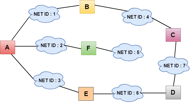
Let’s consider a simplified network consisting of five routers—A, B, C, D, and E. In a Distance Vector algorithm, if Router A wants to send a packet to Router E, it consults its routing table to determine the shortest path. It doesn’t know the entire path from A to E but knows the next hop—say Router B—where it should send the packet for it to eventually reach Router E.
2. Key Concepts and Terminologies
Before diving deeper into the intricacies of the Distance Vector Routing Algorithm, it’s crucial to understand some key terms and concepts that are frequently used in the context of this algorithm. These terminologies will help in a clearer understanding of how Distance Vector works, and they are essential for anyone looking to implement or troubleshoot a network using this routing algorithm.
Routing Table
The routing table is a data structure that resides in a router and keeps track of paths to various network destinations. Each entry in the table consists of, at the very least, a destination network and a ‘next hop’ address, which indicates the next router in the path to that destination. The table is what the router consults to decide where to forward a data packet.
Example:
| Destination | Next Hop  | Metric |
|-------------|-----------|--------|
| 192.0.2.0   | 10.0.0.2  | 2      |
| 203.0.113.0 | 10.0.0.3  | 1      |
Metrics
In the context of Distance Vector, metrics are numerical values used to determine the “distance” to a destination network. Metrics can be calculated based on various factors like hop count, latency, or even manually configured values. A lower metric is generally preferable, as it signifies a more desirable path.
Example:
- Hop Count: Each time a packet passes through a router, the hop count increases by one.
- Latency: Measured in milliseconds, it calculates how long it takes for a packet to reach its destination.
- Bandwidth: It could also use the available bandwidth as a metric, preferring routes with higher bandwidth.
Bellman-Ford Algorithm
The Bellman-Ford Algorithm is the mathematical model that underpins the functionality of many Distance Vector Routing Algorithms. Named after its developers, Richard Bellman and Lester Ford, this algorithm calculates the shortest path to all destinations from a single source, handling even paths with negative weights. In the realm of networking, it is utilized to update the routing table with the best possible paths.
Here’s a simplified step-by-step description:
- Initialize the distance from the source router to all other routers as infinite, except for itself, which is zero.
- For each neighboring router, calculate the distance to every network destination via that neighbor.
- If the newly calculated distance to a destination is shorter than the existing distance, update the routing table.
- Repeat the process until no further updates are made to the table.
By understanding these key terms and concepts—Routing Table, Metrics, and Bellman-Ford Algorithm—you’re now better equipped to grasp the workings and nuances of the Distance Vector Routing Algorithm. In the next sections, we will delve into how these elements play out in real-world applications.
3. How Does Distance Vector Routing Algorithm Work
In this section, we’ll peel back the layers to understand the mechanics behind the Distance Vector Routing Algorithm.
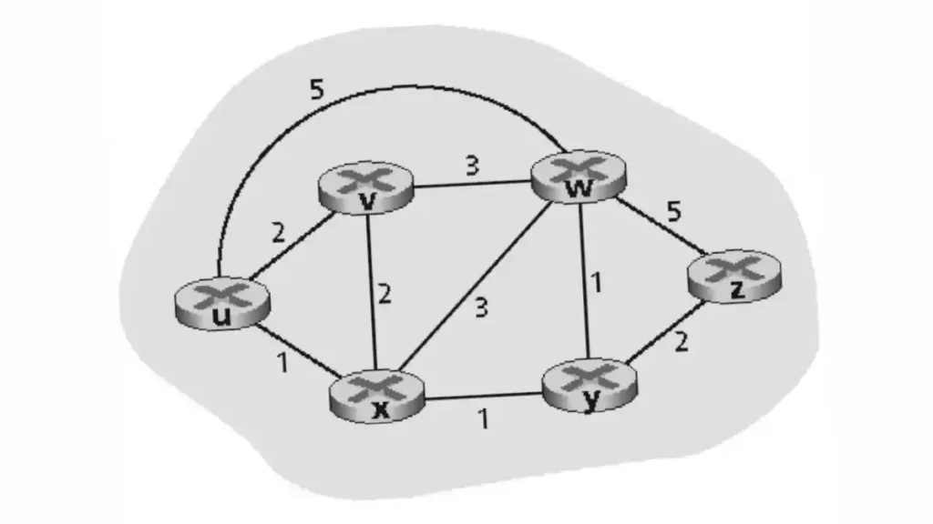
The Distance Vector Routing Algorithm operates on the fundamental principle of periodic table exchanges among neighboring routers. Each router maintains a routing table that contains the shortest distance to every possible destination within the network and the identifier of the neighboring router that will be the next hop for that destination.
Algorithm Steps
- Initialization: When a router boots up, it initializes its routing table with the cost of reaching its immediate neighbors. For unreachable destinations, the cost is set to infinity.
- Table Exchange: Routers periodically send their routing tables to their immediate neighbors. This is done either at regular intervals or when there is a change in the network topology.
- Table Update: Upon receiving a table from a neighbor, a router updates its own table by using the Bellman-Ford equation to calculate the shortest path to each destination.
- Bellman-Ford Equation: New Cost to Destination = Cost to Neighbor + Cost from Neighbor to Destination
- Loop Detection: Techniques like Route Poisoning and Hold-Down timers can be implemented to avoid routing loops.
- Convergence: The algorithm continues the process of table exchange and update until the tables are stable, and no more changes occur. At this point, the algorithm has “converged,” and the routing tables will not change unless there is a change in the network topology.
Routing Table Updates
The frequency of table updates and the method of exchange can vary. Some Distance Vector protocols, such as RIP (Routing Information Protocol), use a timer-based approach where updates are sent every 30 seconds. Others might trigger updates only when there’s a change in the network, thereby reducing bandwidth usage.
Practical Example
Consider a network with four routers: A, B, C, and D. Let’s say a new link is established between C and D. Once this happens, C and D update their tables and share the new information with their neighbors. Eventually, all routers in the network update their tables to reflect this new path, demonstrating how the Distance Vector Routing Algorithm adapts to changes in the network topology.
The following table shows the correspondence between routable network protocols and distance vector routing protocols.
4. Advantages and Disadvantages
In this section, we delve into the pros and cons of employing the Distance Vector Routing Algorithm in your network. Understanding the strengths and weaknesses can guide you in choosing the most appropriate routing algorithm for your specific needs.
Advantages
- Simplicity: The algorithm is simple to understand, implement, and manage, making it a good fit for small to medium-sized networks.
- Low Resource Requirement: Distance Vector protocols typically require less computational power and memory, making them cost-effective for organizations with budget constraints.
- Fast Convergence in Small Networks: In smaller networks with fewer routers, the Distance Vector algorithm can quickly converge to a stable state.
- Autonomous: Each router operates independently, only needing information from its immediate neighbors, reducing the amount of inter-router communication.
Disadvantages
- Scalability Issues: In large networks, the periodic table updates can consume significant bandwidth and slow down convergence times.
- Susceptibility to Routing Loops: The algorithm is prone to routing loops, although techniques like Route Poisoning and Hold-Down timers can mitigate this to some extent.
- Limited Topological Knowledge: Routers have a limited view of the network, knowing only the distance to a destination but not the actual path, which can lead to sub-optimal routing decisions.
- Slow Convergence in Large Networks: In a more complex or larger network, it can take a significant amount of time for the algorithm to converge to a stable state. Learn more about the Slow Convergence Problem.
5. Types of Distance Vector Routing Algorithms
Different flavors of the Distance Vector algorithm have been developed to address its limitations and to tailor it to specific network requirements. Here are some notable ones:
- Routing Information Protocol (RIP): One of the oldest Distance Vector algorithms. It uses hop count as the metric and has a maximum limit of 15 hops.
- Interior Gateway Routing Protocol (IGRP): Developed by Cisco, this proprietary algorithm offers improvements over RIP, like support for multiple metrics including bandwidth, delay, and reliability.
- Enhanced Interior Gateway Routing Protocol (EIGRP): Also by Cisco, EIGRP combines the best of Distance Vector and Link-State algorithms. It’s more efficient and scales well to larger networks.
- Babel: A modern, loop-avoiding Distance Vector protocol designed for mobile and wireless networks.
6. Practical Applications and Use Cases
In this section, we’ll explore where Distance Vector Routing Algorithms shine in real-world scenarios. Understanding these use-cases can guide you in implementing the right routing solution for your specific environment.
Small to Medium-sized Networks
Distance Vector Routing Algorithms are a solid choice for smaller networks with fewer routing devices. Their simplicity and lower computational needs make them well-suited for environments where complex configurations and high computational power are not required.
Backup Routes in Large Enterprises
Even in large networks that primarily use more advanced routing algorithms, Distance Vector can serve as a fallback or backup routing mechanism. This provides an additional layer of resilience, ensuring that network traffic can still be routed in case the primary mechanism fails.
IoT Devices and Networks
The lightweight nature of Distance Vector Routing Algorithms makes them suitable for IoT networks, where devices have limited processing capabilities. They are especially useful in networks where the topology doesn’t change frequently but still requires dynamic routing capabilities.
Mobile Ad Hoc Networks
Modern variants of Distance Vector algorithms like Babel are designed to work well in mobile and ad hoc networks. These are networks where the topology is highly dynamic, and a lightweight, adaptive routing algorithm is needed.
7. References
- Tanenbaum, Andrew S., and David J. Wetherall. “Computer Networks,” 5th ed., Pearson, 2010.
- “RFC 1058 – Routing Information Protocol (RIP),” Internet Engineering Task Force (IETF), June 1988.
- “Cisco: Enhanced Interior Gateway Routing Protocol (EIGRP),” Cisco Systems Inc., Technical Documentation, various years.
- “Babel Routing Protocol,” IETF, RFC 6126, April 2011.
- Request For Comments 1075: Distance Vector Multicast Routing Protocol